Tag Archives: IMU

AVC – Problems

The basic prototype worked on the bench, but as I built it on to the chassis, it started to have issues. The magnetometer would give very random and unreliable readings. I kind of assumed I’ve get some interference, but this was reading north sometimes 180 degree out. In addition, the reading changed when the motors ran and the servos moved. I assumed I was getting magnetic flux from the motors and servos, and this was interfering with the magnetometer. However, without the motors running, I was also getting bad drift from the magnetometer. For example, I would point the car north, take a magnetometer reading, then rotate the car 360 degrees, the reading wouldn’t give me a 360 change. When I get back to north I would read 280 odd degrees, in addition, if I did the same experiment in different places in the room, or at different times, I got different readings. The magnetometer be useless if I couldn’t reliably know where “north” was.

The xBee also had issues, and seemed to only work up to about 1-2m away … which wasn’t very useful. I only had 1mW series 1 devices, which on the data sheet said they’d get 600m, so I expected a bit better than 2m, but I assume this was also due to interference. This wasn’t a deal breaker, as most of the testing could be done with the car no actually driving. All the debugging was around the steering, so 2m was fine to just not have a cable in the way. But it was frustrating … I had to follow the car around carrying the laptop, instead of just sitting in the garden at a table and taking reading as it drove around.

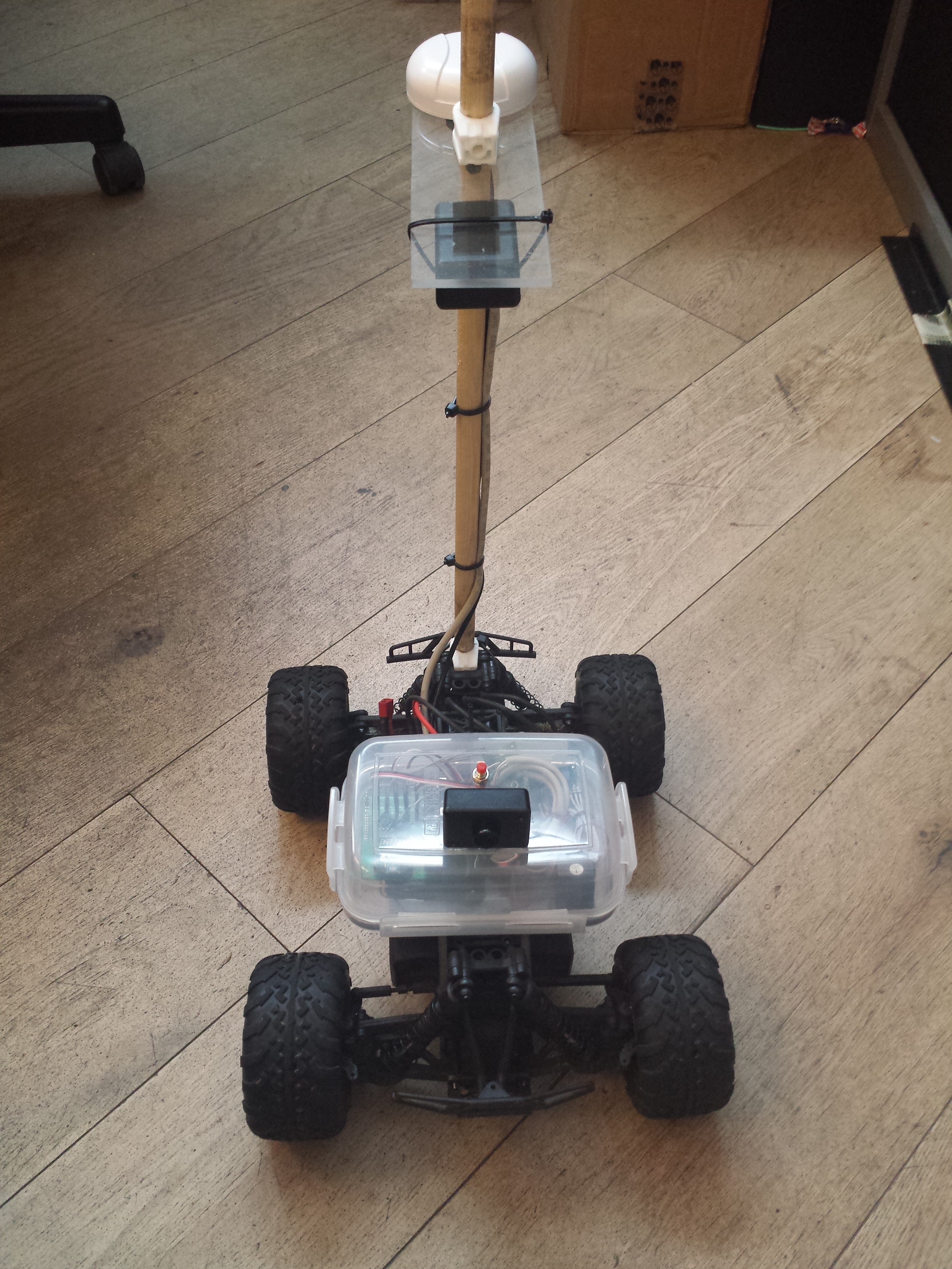
I stuck with the xBee but I moved the magnetometer away from the main board and chassis, to try and reduce the interference. I assumed the interference was magnetic flux coming from the huge brushless motor and large powerful steering servo in the car. If I mounted the magnetometer away from these, perhaps I’d get a more reliable reading. And so was born “broom-handle-bot”

SparkFun AVC 2013 autonomous robot

SparkFun AVC 2013 autonomous robot

While working on the prototype I was also researching better GPS solutions. The basic GPS module I was using only had an accuracy of about 2-5m. This would be tricky to avoid a barrel or hit a jump 1m wide. I had stumbled across SBAS while research GPS issues and this potentially could give me accuracy down to 1-2m. Much better. You can read the wiki page for more details, but effectively (IIUIC) the SBAS system sends a separate signal from a different set of satellites that contains data to improve the accuracy of the main GPS signal. It compensates for atmospheric interface, and other transmission errors. There are different SBAS systems in different parts of the world, WAAS in North America and GLONASS in Europe. I would need a GPS receiver that supported both. Again, with some googling, I found NaviLock and the NL-622MP MD6 GPS Receiver. The data sheet confirmed it supported WAAS and GLONASS, it uses the latest u-Blox chipset, and came in a handy mountable self-contained puck. I ordered one and it arrived. The only downside was the output was RS232 (+/- 15v) not TTL, so I’d need a level shifter board to connect it to the mBed. If I had spent more time looking, they do do a TTL version, which would have been easier …

The very first test of the new GPS puck was transformational. The old GPS wouldn’t get a lock inside my house, which made testing a real pain. I would have to write the code, upload it, then disconnect the system, walk outside in to the garden, test it in the cold, then come back in and debug it, then repeat. This wouldn’t have been so bad, if this was on a Sunday afternoon, but due to my job and family commitments, nearly all my tinkering was done at night, between the hours of 10pm and 2am. It was also the back end of winter, and still snowy some weekend. Testing in the garden at midnight in the snow wasn’t fun.
The new GPS got a lock inside. Plus it got a lock really quickly, within seconds. The old GPS took minutes. It was clear from the first few outside tests that the accuracy was much better and the reading more stable. The GPS used the uBlox 6 chipset, with came with a very detailed and advance desktop config and debug utility.

The basic system was working. However I still had magnetometer issues. The reading would vary wildly if the magnetometer was close to the car. Even if it was some distance way, it wasn’t reliable. It would point north, then I would rotate it 180 and it wouldn’t point S, it would read 160 degrees, then I point it north again and it would read -30. If I rotated it 360 degrees sometimes it didn’t move, sometimes it rotated 250 degrees. I tried lots of different configurations. Even on the bench with no magnets or metal close it wasn’t reliable.
After some extensive Googling, it seemed I need to perform a calibration. This would calibrate out basic interference if the interference was constant, like a steel mounting screw that was always in the same relative position to the sensor. This link explains the process. You take lots of readings from every orientation, imaging mounting the sensor on gimbals and spinning it on all axis, so the tip of the sensor scribes the outline of a sphere. Ideally you want a data cloud of points in all orientations from all three sensors; x, y & z.
Once you have the data set you need to do three things;

  1. You need to remove “erroneous” readings, called outliners. There are clearly (statistically) incorrect. These are obvious to spot manually as the sit outside the circle/sphere of normal readings.
  2. You need to normalise the data in all three axis, so all the maximum readings from all the of the x, y & z sensors have the same magnitude
  3. You need to shift the data so to each set of readings is centred on zero.

Imagine a point cloud that is slightly oval shaped. The normalisation process shifts and scales the cloud so it’s a perfect circle, orgined around zero.These scaling and offset numbers are then used to scale the raw reading to give better accuracy.

Compass Calibration - Before

Compass Calibration – Before

Compass Calibration - After

Compass Calibration – After

This worked to an extent, and the magnetometer was noticeably more accurate and stable, but I still had problems. So I thought I’d tried a different approach. I had an IMU sensor from a previous project. This sensor has 9 DoF (gyro, accelerometer & magnetometer) plus a CPU and contains a kalman filter to process the data. It will give Euler angles, and all I was after was “yaw” – Phi. The issue was the device was not I2C, but serial or SPI. The serial interface had complex packet structure and I didn’t have time to write and debug a parser, so I opted for SPI. I modified the code to read SPI and got a basic Phi reading from the device.
This was more accurate. But it now had a different problem. The issue with yaw calculating with a 9 DoF board, is the yaw cannot use the accelerometer data, as it rotates around the accelerometer axis so it never changes. It can only merge the magnetometer and gyro data. And this is susceptible to gyro drift. This manifested itself in the yaw reading slowing rotating even when the unit was stationary. There was a function in the devices to zero the gyros when the unit was at a known stationary position, but after time the drift returned. That clearly wasn’t going to work.

The final option was to try the same basic magnetometer code, but with these IMU magnetometer readings. You can read all the raw gyro, accelerometer, magnetometer readings, plus the processed (filtered) version, plus the Euler angles from the device.
It turned out the process (filtered) raw magnetometer readings were pretty stable. So I had my final solution. However … about a week before the competition!

Other posts in this series :

AVC – It’s ready !

It’s ready ! My entry for the Autonomous Vehicle Competition in the US next week is built and (partially) tested. I’ve entered the Autonomous Vehicle Competition run by SparkFun Electronics, held in Boulder, Colorado. See : http://avc.sparkfun.com & http://www.sparkfun.com

Tupperware Bot !

Tupperware Bot !

I’ll do a series of more detailed posts after I come back, but here is a brief synopsis.

It’s an HPi Savage Flux XS radio controlled car underneath (The “world’s fastest mini monster truck”) It will do 55 MPH on a good day, but I won’t be running it anywhere near that fast. The brain is an mBed (ARM base microcontroller). Attached is a high accuracy GPS (I’m getting about 1.5-2m accuracy using SBAS), an electronic compass (So I know which way the car is pointing), an ultrasound range finder (to sense obstacles) and a big red “go” button ! 🙂

The mBed ingests the GPS data, range finder and compass data and works out where it’s currently pointing and the delta to where it needs to point to reach the next waypoint. The delta is fed in to a PID control algorithm that controls the steering servo. Currently the speed controller is a static speed (slow) but as I get more confidence in the testing, it will be proportional to the distance from the next waypoint (i.e. faster, then slowing as you near the turn point.) The range finder is processed and inserts an offset in to the PID control input if it detects an obstacle, to try and steer round it.

Other posts in this series :

BalanceBot – Arduino Code

With the use of the various libraries the main code loop is very simple. Once all the objects are initialised, the loop reads the robots angle, computes the PID output and uses that to set the motor speed and direction.

void loop()
{
my3IMU.getYawPitchRoll(ypr);
Input = ypr[IMU_ROLL];
myPID.Compute();
md.setSpeeds(Output,Output);
}

The system worked (ish). As mentioned previously, it took a while to find the PID parameters, and they are still not perfect. However I did get a problem.

The robot would balance, but after a few minutes, both motors would just turn on full. Sometimes one motor. The strange thing was sometimes the other motor would still be managed by the PID algorithm, and would change direction when the robot was tilted back and forth, so it wasn’t as if the Arduino had crashed. I initially thought there was a short circuit or lose connection but I couldn’t find one.

I had trouble in the past with other projects, where the code is large and complex, the Arduino sometimes exhibits strange behaviour. Not quite crashing, but being erroneous. I has a suspicion the device is running out of RAM. The programs either had too many variables, or too many recursive functions. I’ve not researched a way to model programs to estimate their RAM usage, or if there is a way to report RAM usage via the code. I’m sure there’s a way. Let me know if you have any ideas.

So, I just threw hardware at the issue, and upgraded the Arduino with a Mega, which has four times the RAM (8k on the Mega verses 2k on the Uno). This solved the problem immediately. Whereas the robot would “crash” every time on the Uno, the same code worked without any issue on the Mega.

One problem was the Mega though is it’s physically longer, so it sticks out of the side of the robot 😦

The other issue was the SPI and TWI pins on the Mega are on different pins to the Uno. Not a huge problem, but until I update the shield PCB, it means jumper wires.

Full code listing below:

#include <ADXL345.h>
#include <HMC58X3.h>
#include <ITG3200.h>
#include <Wire.h>
#include <EEPROM.h>
#include <FreeIMU.h>
#include <CommunicationUtils.h>
#include <DualVNH5019MotorShield.h>
#include <SPI.h>
#include <PID_v1.h>

//#define DEBUG
#include <DebugUtils.h>

// *** Duemilanova / Uno
// IMU uses I2C - pins A4 (SDA) & A5 (SCL)
// Quad counter uses SPI - pins D11 (MOSI), D12 (MISO) & D13 (SCK)

// *** Mega 2560
// IMU uses I2C - pins 20 (SDA) & 21 (SCL).
// Quad counter uses SPI - pins D50 (MISO), D51 (MOSI) & D52 (SCK)

// IMU constansts
#define IMU_YAW 0
#define IMU_PITCH 1
#define IMU_ROLL 2

#define Ku 20    // where is oscilates
#define Pu 0.4   // period of oscilation
#define Kp 0.6 * Ku
#define Ki (2 * Kp) / Pu
#define Kd (Kp * Pu) / 8

//IMU variables
float ypr[3]; // yaw/pitch/roll
FreeIMU my3IMU = FreeIMU();

//PID variables
double Setpoint, Input, Output;
PID myPID(&Input, &Output, &Setpoint, Kp, Ki, Kd, DIRECT); //or REVERSE

//MotorDriver
DualVNH5019MotorShield md;

void setup()
 {
  Serial.begin(115200);

  // Initialise Motor Driver:
  Serial.println("#Init Motor Driver");
  md.init();
  delay(50);

  // Initialise Wire Library:
  Serial.println("#Init Wire library");
  Wire.begin();
  delay(50);

  // Initialise SPI:
  Serial.println("#Init SPI library");
  SPI.begin();
  SPI.setDataMode(SPI_MODE0);
  SPI.setBitOrder(MSBFIRST);
  SPI.setClockDivider(SPI_CLOCK_DIV8);
  delay(50);

  // Initialise IMU:
  Serial.println("#Init IMU");
  my3IMU.init();
  delay(50);

  // Get Initial variables:
  Serial.println("#Get first YPR");
  my3IMU.getYawPitchRoll(ypr);

  // Initialise PID:
  Serial.println("#Set initial Input variable");
  Input = ypr[IMU_ROLL];
  Serial.println("#Init IMU Setpoint");
  Setpoint = 0;
  myPID.SetMode(AUTOMATIC);
  myPID.SetOutputLimits(-400,400);

  Serial.println("#Exit Setup");
}

void loop()
{
  my3IMU.getYawPitchRoll(ypr);
  Input = ypr[IMU_ROLL];
  myPID.Compute();
  md.setSpeeds(Output,Output);
  stopIfFault();
}

void stopIfFault()
{
  if (md.getM1Fault())
  {
    Serial.println("#M1 fault");
    while(1);
  }
  if (md.getM2Fault())
  {
    Serial.println("#M2 fault");
    while(1);
  }
}

BalanceBot – PID Controller

A  PID Controller is a software algorithm typically used to control industrial processes. A PID Controller (Proportional Integral Derivative Controller) calculates the difference between a measured variable and a desired set point. The controller attempts to minimize the error by adjusting the input.

A good example of why a PID Controller is better than other methods of control, is an electric oven. The input is the power to the heating element, the output is the temperature and the set point is the desired temperature.

Without a PID controller, If you turn the power on and off using a simple thermostat, when the temperature of the oven reaches the set point the oven will over shoot the temperature as there is residual heat left in the heating element. If you want the temperature of the oven to be 200 degrees, and have the element fully on until it reaches 200 degrees, then turn it fully off, the temperature will overshoot to maybe 205 degrees, then slowly cool until it reached 199 degrees when it will turn fully on again, however it will take time to heat up, in which time the oven has cooled to 195 degrees, and so it repeats. The oven will oscillate between 195 and 205 degrees, and not actually be a steady 200. This is fine for cooking sausages, but no good for a delicate chemical process.

The PID Controller has three values; the Proportional, the Integral and the Derivative values, denoted P, I, and D. Heuristically, these values can be interpreted in terms of time: P depends on the present error, I depends on the accumulation of past errors, and D is a prediction of future errors, based on current rate of change. By combining the three terms continuously the algorithm maintains the desired set point with minimal errors.

Simple huh ? Well kind of… The maths is a bit complex, but again, there are existing libraries that do it for you. On the Arduino site you can download a fully working PID Controller library, to integrate in to your project : http://playground.arduino.cc/Code/PIDLibrary

The only problem is you need to “tune” a PID Controller to your specific application. The P, I & D terms will be different for an oven, chemical tank, or balancing robot. There are lots of ways of tuning a PID Controller, from mathematical, to trial and error. A control systems friend of mine recommended I try the Ziegler–Nichols method.

The Ziegler–Nichols tuning method is as follows;

  • The P, I & D terms are referred to as “gains” Kp, Ki & Kd.
  • The Ki and Kd terms are first set to zero.
  • The Kp term is manually increased until the robot reaches the ultimate gain, Ku, at which point the it starts to oscillate.
  • The oscillation period Pu is measured and used to set the PID terms as follows :
  • Kp = 0.6 * Ku
  • Ki = (2 * Kp) / Pu
  • Kd = (Kp * Pu) / 8

This isn’t perfectly tuned to our specific system, but it’s a good approximation. PID tuning is a black art that requires a lot of knowledge and skill. This will do for the time being.

I am using the tilt angle of the robot as the input and the speed of the motors as the output.

The code is quite simple. The three variables are all floating point numbers.

double Setpoint, Input, Output;

The PID object is instantiated with the three PID values I calculated from my Ziegler–Nichols tuning method

PID myPID(&Input, &Output, &Setpoint, Kp, Ki, Kd, DIRECT);

The desired set point is 0 degrees, i.e. the robot is perfectly upright

Setpoint = 0;

Then in my main loop I get the angle of the robot, run the PID compute function, and using the output set the motor speeds.

void loop() {
  my3IMU.getYawPitchRoll(ypr);
  Input = ypr[IMU_ROLL];
  myPID.Compute();
  md.setSpeeds(Output, Output);
}

That’s the theory anyway … the results were mixed. It took a number of attempts to find the oscillation gain and period (Ku & Pu) accurately. And with those values, the PID controller wouldn’t balance the robot. It took lots of manually trial and error of various values to find something that was stable. PID tuning is very much a black art.

I did get it to balance though and it was more stable that the equivalent “cubed” algorithm I was using. However with the IMU code and the PID code on the Arduino, I started getting problems with the Arduino crashing. I can only assume it was running out of RAM.

I switched to an Arduino Mega and everything worked fine. So I’ve stuck with that for the time being. The Mega is much more stable, however the custom PCBs I made don’t fit the Mega, so the wiring is messy, plus the Mega sticks out of the frame. Next job is to make the PCB as a Mega Shield and turn the board round long ways so it fits better.

The PID controller is still not perfect, but it’s relatively stable. You can see it recovers from oscillation, which the basic controller didn’t. But It still drifts badly, and still falls over eventually. But progress none the less.I need to get the Quadrature decoders working so I can stop the drifting.

Here’s a short video of the PID Controlled BalanaceBot in action.

BalanceBot – Sensors and IMU Library

The BalanceBot needs to know if it’s upright to balance. If it starts tipping over in one direction the robot needs to sense how far it has tipped over and speed up the motors in that direction to counter the tipping motion. This will compensate for the tipping motion by driving the bottom of the robot under its centre of gravity and stand it back upright again.

Sensing the angle of the robot on a simple level could be achieved with a single g-force sensor or accelerometer. The accelerometer measures acceleration. Our planets gravity, acting on an object, is acceleration, so the accelerometer can be used to measure gravity. Gravity always pulls down towards ground at a constant value. By knowing the value you can calculate the angle of the sensor. If the sensor reads 1g, the sensor is “vertical” with the ground. If the accelerometer reads 0g the sensor is “horizontal” with the ground. By using trigonometry, the value of g can be used to calculate any angle of the sensor.

However this is only true if the sensor is perfectly still, and the only acceleration acting on it is gravity. As we are going to mount this in a moving robot, the acceleration of the robot will cause the accelerometer to read not just the gravitational force, but also any acceleration of the robot, which will render the reading inaccurate when calculating the angle of the robot.

Another method of measuring the angle of the robot is with a gyroscope. A gyroscope measures rotation velocity around an axis. If you know the angle of the sensor to start with, then continuously measure the rate at which it rotates, you can calculate the current angle. This has two issues; firstly you need to know your angle to start with and secondly any error in the calculation is compounded with time, so the calculated value “drifts” over time and become less accurate. However a gyroscope is immune to interface from acceleration.

So, if you can combine the accelerometer data and gyroscope data together you can use both readings to compensate for the inaccuracies of the other. The accelerometers can compensate for the gyroscope drift as they give exact readings at a known time. The gyroscopes compensate for the non-gravitational acceleration as they only measure rotation velocity.

This process is called “sensor fusion”. There are lots of method of processing the accelerometer and gyroscope data to give a single accurate angular reading. These include Kalman Filters and Complimentary Filters. The maths can get a bit complex but it’s all based on trigonometry. You could write your own code, but there are lots of existing, tested, libraries that do this for you.

Using such a library and the appropriate sensor can give your orientation in 3D space, your Roll, Pitch and Yaw angles, or Euler Angles. This traditionally uses an additional sensor to measure yaw, as yaw cannot be measured with a g sensor, as yaw rotates around the vertical axis, and so the force of gravity doesn’t change. The easiest way to measure yaw is with a magnetometer, this measures the earth magnetic field and can calculate your orientation to “North” (magnetic north).

BalanceBot IMU - Sparkfun 9 DOF sensor stick.

BalanceBot IMU – Sparkfun 9 DOF sensor stick.

The individual sensors all work in a single plane, so a single gyroscope only measures rotational velocity in one direction. An accelerometer only measures acceleration in one direction. Depending on how much your sensor, or robot, moves, you may need three of each sensor in each orientation (x, y & z) to calculate your orientation in 3D space. For example, as the “X” axis accelerometer rotates it will no longer be vertical and will become horizontal at which point, depending on the orientation, of the sensor either the “Y” or “Z” accelerometer begin to point down. Using 3D trigonometry of the X, Y & Z accelerometer reading, you can begin to calculate the orientation in 360 degrees. This is called “three degrees of freedom” you are measuring 3 independent parameters that define its orientation. If you add three gyroscopes, and three magnetometers, you end up with 9 Degrees of Freedom, or 9DOF.

Using a 9DOF sensor and a maths library, you can calculate (almost) any orientation accurately. This combination of sensors and maths is called an Inertial Measurement Unit or IMU. There are lots of these, ranging in accuracy and cost. They can cost thousands of pounds. However there are lots of hobby level devices too for less than £100.

You have the choice of separate sensors and use your own CPU for the maths, or use an all in one device that includes its own CPU. I have an UM6-LT Orientation Sensor from CH Robotics for a different project. They are easy to interface to and do all the Kalman filtering for you on board and provide the filtered, stable Euler Angles via a serial interface. However I was using this device in a different project.

There are many 9 DoF boards containing just the sensors. FreeIMU is a popular board, cheap and compact. SparkFun produce a 9DoF Sensor Stick which I decided on, as its cheap, small and easy to interface to.

The FreeIMU site provides a GNU GPL license library for Arduino which supports not only the FreeIMU boards but also the SparkFun boards and the DIYDrones ArduIMU. This provided the sensor fusion calculations to provide a stable combined output from the raw sensors.

The SparkFun board uses an I2C interface to communicate with the Arduino. This is a bidirectional serial interface, using just two data wires, and power.

To be clear I didn’t need a 9DOF board in this simple robot, as I only needed to calculate the robots orientation in one axis (the axis that rotates around the wheels) however, by using a 9DOF board I get full 3D orientation which means it doesn’t matter which direction I mount the sensor in, plus I intend to use the magnetometer reading to capture the “heading” the robot is traveling on so I can make it travel in a straight line. It was also fun to learn.

There are two common ways to represent a 3D orientation; Euler Angles and Quaternions.

Euler Angles can be understood easily if you imagine an old fashioned gyroscope in an aeroplane. A spinning mass is suspended in space on 3 gimbal bearings, that each rotate in a perpendicular axis. As the aeroplane tilts left and right (rolls) the gimbals rotate to keep the mass level. This angle of roll is the Roll Euler Angle. Same for Pitch, the movement of the nose of the plane up and down, and Yaw the rotation of the plane caused by the movement of the rudder. These three Euler angles define the Roll, Pitch and Yaw of the object. However Euler Angles have a flaw, as one of the axis rotates 90 degrees, it aligns with one of the other axis. In fact all three axis can align. This is called Gimbal Lock.

Gimbal lock is the loss of one degree of freedom in a three-dimensional space that occurs when the axes of two of the three gimbals are driven into a parallel configuration, “locking” the system into rotation in a degenerate two-dimensional space.

This means in some situations Euler Angles cannot accurately define our orientation. However they work fine for movements that do not exceed 90 degree rotations, which is our case if fine, as we will only be “wobbling” a few degrees from vertical. (I hope)

An alternative system is called Quaternions which does not suffer from Gimbal Lock. This uses imaginary numbers to define our three dimensional orientation, and is way too complex to try and explain here. Plus I don’t really understand it enough 🙂

So, I stuck with Euler Angles.

The FreeIMU library provides a simple function to calculate the Euler Angles :

my3IMU.getYawPitchRoll(ypr);

This fills a 3 dimensional variable with three floating point numbers, which contains the Pitch, Roll and Yaw angles.

With my sensor mounted as it is, the “Roll” angle is the rotation around the wheels, this is the only value I use:

angle = ypr[IMU_ROLL];

With just this value I can balance the robot. If the angle is positive, I drive the wheels in one directions and it the angle is negative I drive the wheels in the other direction. By proportionally driving the wheel speed, relative to the angle, the robot balances. I tested it using a cube function. i.e. Speed = Angle ^ 3

If the angle is 1 degree, the speed is 1 (slow), if the angle is 2 degrees the speed is 8 (faster), if the angle is 3 degrees the speed is 27 (quite quick), etc. The more the robot falls over the faster the wheels rotate to stand it back up. When the robot is upright the speed is very slow so the robot doesn’t overshoot and start to oscillate.

Of course it does oscillate with this very simplistic control algorithm and falls over. We need a more complicated control algorithm to stop the oscillation.

A PID Controller works well. More on that next…